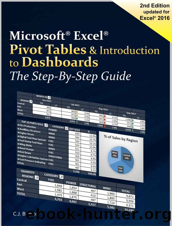
Excel Pivot Tables & Introduction To Dashboards The Step-By-Step Guide by C.J. Benton

Author:C.J. Benton [Benton, C.J.]
Language: eng
Format: azw3
Published: 2017-01-01T16:00:00+00:00

Click the ‘OK’ button

Repeat steps #6 & #7 for cell ‘B11’ (DO NOT REPEAT FOR CELL ‘B26’)

Select cell ‘X27’ (Total TTL), right-click and select ‘Remove Grand Total’

From the Ribbon select the ‘VIEW’ tab and uncheck the ‘Gridlines’ box

Click cell ‘A3’, and then from the PivotTable Tools Ribbon select the tab DESIGN : PivotTable Styles

From the PivotTable Styles drop-down, select a format style you like

Repeat steps #11 & #12 for PivotTables in cells ‘A11’ & ‘A26’

In cell ‘A1’ enter the text ‘Monthly Dashboard’

In cell ‘B1’ enter the text ‘Airplane Parts by Region’

Increase the font size of ‘A1’ & ‘B1’ to 18 and bold, optionally you may change the font type to ‘Consolas’ and color of your choice

Right-click on cell ‘A3’ and from the pop-up menu select ‘PivotTable Options’

Download

Copyright Disclaimer:
This site does not store any files on its server. We only index and link to content provided by other sites. Please contact the content providers to delete copyright contents if any and email us, we'll remove relevant links or contents immediately.